Implemented S3 methods for objects of class "cv.corila":
coef(): extracts estimated coefficients
predict(): calculates predicted values
fitted(): extracts fitted values
residuals(): calculates deviance residuals
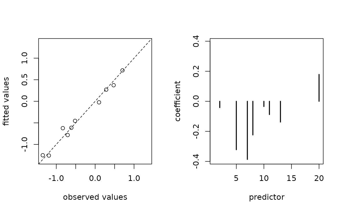
plot(): visualises observed vs fitted values and estimated coefficients
print(): prints information to the console
summary(): summarises the fitted model
deviance(): extracts the deviance
nobs(): extracts the number of observations
Value
coef() returns a \((1 +) p\)-dimensional vector, predict() returns an \(n_1\)-dimensional vector, fitted() and residuals() return an \(n_0\)-dimensional vector. See individual methods for details.
See also
Use cv.corila() to fit the model.
Examples
# listing S3 methods
methods(class = "cv.corila")
#> [1] coef deviance fitted nobs plot predict print
#> [8] residuals summary
#> see '?methods' for accessing help and source code
# simulating data
n <- 10L; p <- 20L; q <- 5L
x <- matrix(rnorm(n * p), nrow = n , ncol = p)
y <- rnorm(n)
group <- rep(seq_len(q), length.out = p)
primary <- as.logical(rbinom(n = p, size = 1L, prob = 0.5))
# fitting the model
object <- cv.corila(x = x, y = y, group = group, primary = primary)
#> Warning: Option grouped=FALSE enforced in cv.glmnet, since < 3 observations per fold
#> wgt_local exp_local wgt_global exp_global threshold cvm
#> 11 1 0 0 Inf 0 5.038443
# using S3 methods
coef(object)
#> (intercept) <NA> <NA> <NA> <NA> <NA>
#> -0.1965035 0.0000000 0.0000000 0.0000000 0.0000000 0.0000000
#> <NA> <NA> <NA> <NA> <NA> <NA>
#> 0.0000000 0.0000000 0.0000000 0.0000000 0.0000000 0.0000000
#> <NA> <NA> <NA> <NA> <NA> <NA>
#> 0.0000000 0.0000000 0.0000000 0.0000000 0.0000000 0.0000000
#> <NA> <NA> <NA>
#> 0.0000000 0.0000000 0.0000000
predict(object, newx = x)
#> [1] -0.1965035 -0.1965035 -0.1965035 -0.1965035 -0.1965035 -0.1965035
#> [7] -0.1965035 -0.1965035 -0.1965035 -0.1965035
fitted(object)
#> [1] -0.1965035 -0.1965035 -0.1965035 -0.1965035 -0.1965035 -0.1965035
#> [7] -0.1965035 -0.1965035 -0.1965035 -0.1965035
residuals(object)
#> [1] 1.5121996 0.8554382 -0.8744874 -0.3424830 -1.1008847 0.3867370
#> [7] -3.3430825 1.4079011 0.4873873 1.0112744
plot(object)
 print(object)
#> object of class ‘cv.corila’
#> (contains multiple objects of class ‘cv.glmnet’)
#> selected 0 from 20 predictors
summary(object)
#> --- object of class “cv.corila” ---
#> generalised linear model with gaussian family
#> 20 features (6 primary and 14 auxiliary features)
#> initial coefficients: ridge regression
#> final coefficients: adaptive lasso regression
#> optimised regularisation parameter: lambda.min = 1.332
#> selected weights: local = 1, global = 0
#> selected exponents: local = 0, global = Inf
#> 1 non-zero coefficients (including intercept)
print(object)
#> object of class ‘cv.corila’
#> (contains multiple objects of class ‘cv.glmnet’)
#> selected 0 from 20 predictors
summary(object)
#> --- object of class “cv.corila” ---
#> generalised linear model with gaussian family
#> 20 features (6 primary and 14 auxiliary features)
#> initial coefficients: ridge regression
#> final coefficients: adaptive lasso regression
#> optimised regularisation parameter: lambda.min = 1.332
#> selected weights: local = 1, global = 0
#> selected exponents: local = 0, global = Inf
#> 1 non-zero coefficients (including intercept)