Fitted values

Extracts fitted values.

Usage

# S3 method for class 'cv.corila'
fitted(object, ...)

Arguments

object

object of class "cv.corila"

...

(for compatibility with stats::fitted)

Value

Returns a numeric vector of length \(n_0\) (one entry for each training observation).

See also

Use predict() to obtain predicted values (i.e., for testing observations).

Examples

# listing S3 methods
methods(class = "cv.corila")
#> [1] coef      deviance  fitted    nobs      plot      predict   print    
#> [8] residuals summary  
#> see '?methods' for accessing help and source code

# simulating data
n <- 10L; p <- 20L; q <- 5L
x <- matrix(rnorm(n * p), nrow = n , ncol = p)
y <- rnorm(n)
group <- rep(seq_len(q), length.out = p)
primary <- as.logical(rbinom(n = p, size = 1L, prob = 0.5))

# fitting the model
object <- cv.corila(x = x, y = y, group = group, primary = primary)
#> Warning: Option grouped=FALSE enforced in cv.glmnet, since < 3 observations per fold
#>   wgt_local exp_local wgt_global exp_global threshold      cvm
#> 1         0       Inf          1          2         0 3.834771

# using S3 methods
coef(object)
#>  (intercept)         <NA>         <NA>         <NA>         <NA>         <NA> 
#>  0.025741927  0.000000000  0.000000000  0.000000000  0.000000000  0.000000000 
#>         <NA>         <NA>         <NA>         <NA>         <NA>         <NA> 
#>  0.000000000  0.000000000  0.000000000  0.000000000  0.000000000  0.000000000 
#>         <NA>         <NA>         <NA>         <NA>         <NA>         <NA> 
#>  0.000000000  0.006990749  0.000000000 -0.222786829  0.000000000  0.000000000 
#>         <NA>         <NA>         <NA> 
#> -0.096166742  0.000000000  0.000000000 
predict(object, newx = x)
#>  [1] -0.3197090  0.1992349 -0.3350059 -0.4794660  0.4194854  0.1101963
#>  [7]  0.3779235 -0.1674397  0.2305534  0.6043664
fitted(object)
#>  [1] -0.3197090  0.1992349 -0.3350059 -0.4794660  0.4194854  0.1101963
#>  [7]  0.3779235 -0.1674397  0.2305534  0.6043664
residuals(object)
#>  [1] -0.10627239  0.79742391  1.06266662 -1.24716457 -0.06608691  0.61661735
#>  [7]  0.29033749 -2.25687765 -0.46591080  1.37526695
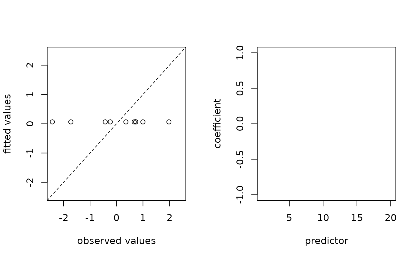
plot(object)

print(object)
#> object of class ‘cv.corila’ 
#> (contains multiple objects of class ‘cv.glmnet’)
#> selected 3 from 20 predictors
summary(object)
#> --- object of class “cv.corila” --- 
#> generalised linear model with gaussian family 
#> 20 features (10 primary and 10 auxiliary features)
#> initial coefficients: ridge regression 
#> final coefficients: adaptive lasso regression 
#> optimised regularisation parameter: lambda.min = 44.02 
#> selected weights: local = 0, global = 1
#> selected exponents: local = Inf, global = 2
#> 4 non-zero coefficients (including intercept)